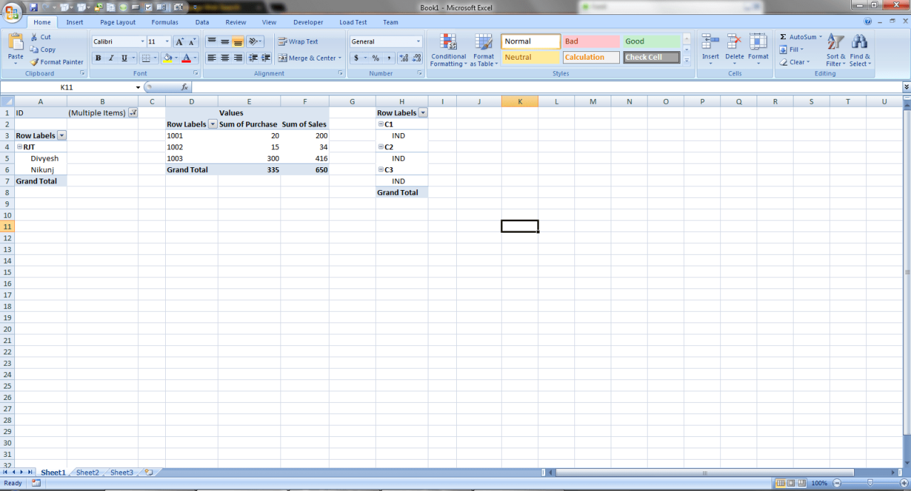
However, If I Add Multiple Rows, The Pivot Tables Grow.

Select a location where the pivottable should be created. On the ribbon, click the insert tab. Now, the table that appears on the screen has the data from all the 4 sheets.

Create A Chart Based On Your First Sheet.

Then, select two ranges, and enter the same name, such as h1. Select “multiple consolidation ranges” in that dialog. We will then press p to activate the pivot table wizard.

I Have Attached A Workbook With An Example.

This will enable the pivot table wizard, as shown below. The alternative is to copy and paste values and. We’ll link a slicer between two data sets in the sections below.the first data set is for the sales data.

For More Information, See Add Worksheet Data To A Data Model Using A Linked Table, Create A Relationship Between Two Tables, And Create Relationships In Diagram View.

But if you want a second chart that is independent from the first chart, you need to create a new pivot table and chart. I have successfully created a pivot table by using vba, but now i would like to create two pivot tables in two separate worksheets, 2 and 3. Choose the applicable table you'd like to create pivotcharts from.

Keep It Pressed Then Click The D Key Then The P Key And You Will See This:

Alt + d is the access key for ms excel, and after that, by pressing p after that, we’ll enter to the pivot table and pivot chart wizard. 8 steps to connect slicer to multiple pivot tables from different data source. We will check the sections as shown in figure 3 and click next.