Lesson plans on manners are also a useful segue into other units in the classroom and a good way to start off the year and establish classroom rules. This social studies worksheet is a great way to facilitate a conversation about social skills with your preschooler.
Free Printable Worksheets About Good Manners Free Printable Worksheets About Manners Preschool Teacher Favorite Things Good Manners
Worksheets and no prep teaching resources values and manners social skills.

Worksheets activities printable worksheets good manners worksheets. This unit is great for any time during the year. Some of the worksheets for this concept are be a manners detective good manners good manners successful social studies kindergarten say please the book of good manners dining etiquette 01 using good telephone etiquette. Free good manners activities and classroom resources.
Teacher planet good manners lessons worksheets and activities by signing up you agree to our privacy policy. Show more details. Writing prompts poem booklet game posters emergent readers and more.
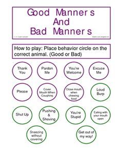
In this manners worksheet little learners will look at two different scenarios and choose which picture shows good manners and which shows bad manners. Use this character education resource to teach students positive social skills and the importance of having good manners. Good manners activities worksheets printables and lesson plans.
Vba sheet xlveryhidden worksheet xlsx vba vba sheet xlsheetveryhidden vba worksheet zoom vba sheet zoom level vba worksheet zuweisen vba worksheets zählen vba sheet zuweisen vba worksheet variable zuweisen excel vba worksheet zuweisen auf worksheet zugreifen vba vba zu worksheet wechseln excel vba worksheet zugreifen vba worksheet. Make 25 types of printable worksheet or use our new interactive e worksheet maker to make digital worksheets. Good manners word search worksheet has 1word search with 23 words words are from left to right right to left upto down and down to up in the wordsearches children across all age groups just love wordsearch challenges.
Once you find your worksheet click on pop out icon or print icon to worksheet to print or download. Sep 12 2016 free printable worksheets about good manners free printable worksheets about. From lessons in common courtesy role playing and manners games printables and worksheets you can pick and choose which lessons you want to teach or emphasize.
Manners worksheets the clever printable and digital worksheet maker from just 3 33 p m quickworksheets is the smart cloud based worksheet generator for making fun effective lesson materials.

Free Printable Worksheets Archives Page 9 Of 14 E Classroom F Social Studies Worksheets Free Printable Worksheets Kindergarten Worksheets Free Printables

Results For Kindergarten Worksheets Social Studies Guest The Mailbox Kindergarten Classroom Rules Kindergarten Social Studies School Worksheets

Manners Activities For Kids Caillou Great Big Book Of Little Wee Games Printable Activities Manners For Kids Table Manners Manners Preschool

Personal Hygiene Worksheet 9 Science Worksheets Grade 2 Worksheets Personal Hygiene Worksheets Healthy Habits For Kids Worksheets For Kids

Teaching Children Manners Worksheets Free Templates Png 1275 1650 Table Manners Kindergarten Worksheets Printable Worksheets

Members Only E Classroom Free Education Worksheets For Schools Health Lesson Plans Hygiene Lessons 1st Grade Worksheets

Teaching Good Table Manners For Better Social Skills During The Holidays And A Social App Gift Giveaw Good Table Manners Table Manners Social Skills Activities

Image Result For Healthy And Unhealthy Habits Worksheet Healthy Habits Kindergarten Healthy Habits For Kids Healthy And Unhealthy Food

Manners Printable Manners Chart And Learning Video Manners Chart Manners For Kids Teaching Manners

Manners Worksheet Education Com Preschool Social Skills Social Skills Manners

Worksheets For Kindergarten Good Manners In 2020 Manners Preschool Manners For Kids Teaching Manners
See The Source Image Manners For Kids Teaching Kids Manners Kids Worksheets Printables

Healthy Habits Www Greennutrilabs Com Healthy Habits For Kids Good Habits For Kids Worksheets For Kids

Image Result For Free Printable Manners Worksheets Manners For Kids Teaching Kids Manners Kids Worksheets Printables

Free Worksheets On Manners Download It Activity Fun Worksheets Activity Sets Worksheets Manners Fun Worksheets Worksheets Free Manners Activities

Manners Match It Up Worksheet Freebie Girl Scout Activities Social Skills Groups Social Skills

Good Manners Worksheet Good Manners Activity Good Manners Kindergarten Manners Activities Have Fun Teaching Good Manners

Preschool Free Worksheets Good Manners Manners Preschool Preschool Worksheets Kindergarten Worksheets Printable

English Teaching Worksheets Healthy Habits Teaching Healthy Habits Healthy Habits Preschool Healthy Habits For Kids